

Discover the Magic of Descriptive Statistics Using Python
In today's data-driven world, making sense of raw data is more important than ever. Whether you're a beginner in data science or a seasoned analyst, understanding descriptive statistics using Python is a crucial skill for effective data analysis. Descriptive statistics help summarize and interpret complex datasets through meaningful metrics like mean, median, mode, and standard deviation.
In this guide, you’ll learn how to unlock powerful insights using Python’s most popular libraries, including Pandas, NumPy, and SciPy. We’ll walk through real-world examples, step-by-step code, and visualizations to help you quickly grasp the fundamentals and apply them in your own projects.
By the end of this post, you'll not only understand what descriptive statistics are but also how to use them efficiently with Python to reveal patterns, spot outliers, and tell compelling data stories.
Table of Contents
Understanding Measures of Central Tendency in Python
When analyzing any dataset, one of the first steps is to understand its central values the points around which data tend to cluster. These are known as the measures of central tendency, and they include the mean, median, and mode. Each of these statistics provides a different perspective on what a “typical” value looks like in your data.
In this section, you'll learn how to calculate and interpret the mean, median, and mode using Python. We'll use real-world examples and Python libraries like pandas to demonstrate how these measures can help summarize your data quickly and effectively.
How to Calculate the mean in Python
The mean, often referred to as the average, is one of the most commonly used measures of central tendency. It represents the sum of all values in a dataset divided by the number of observations.
\bar{x} = \frac{1}{n} \sum_{i=1}^{n} x_i
\)
With:
\(\bar{x}= \hspace{0.5em} The \hspace{0.5em} mean \hspace{0.5em} (average) \\
n= \hspace{0.5em} Number \hspace{0.5em} of \hspace{0.5em} data \hspace{0.5em} points \\
x_i= \hspace{0.5em}Each \hspace{0.5em} individual \hspace{0.5em} value \hspace{0.5em} in \hspace{0.5em} the \hspace{0.5em} dataset \\
\)
In Python, calculating the mean is simple and efficient using libraries like NumPy and Pandas.
import pandas as pd
import numpy as np

# Sample data: Monthly sales figures
monthly_sales = [220, 270, 250, 300, 310, 280, 260]

# Using NumPy
mean_numpy = np.mean(monthly_sales)
print("Mean using NumPy:", mean_numpy)

# Using Pandas
sales_series = pd.Series(monthly_sales)
mean_pandas = sales_series.mean()
print("Mean using Pandas:", mean_pandas)

#Output:
# Mean using NumPy: 270.0
# Mean using Pandas: 270.0
As shown above, both NumPy and Pandas return the same result. The mean gives us a quick sense of the typical value in the dataset, making it useful for comparing groups or tracking trends over time. However, keep in mind that the mean can be influenced by extreme values (outliers), which is why it’s often used in conjunction with the median.
How to Calculate the median in Python
The median is the middle value in a sorted dataset. It’s especially useful when your data contains outliers or is skewed, as it represents the central tendency more accurately than the mean in those cases. For example, in income data where a few extremely high values can inflate the mean, the median gives a better sense of what a “typical” value looks like.
\text{Median} =
\begin{cases}
x_{\left(\frac{n+1}{2}\right)} & \text{if } n \text{ is odd} \\
\frac{1}{2} \left( x_{\left(\frac{n}{2}\right)} + x_{\left(\frac{n}{2} + 1\right)} \right) & \text{if } n \text{ is even}
\end{cases}
\)
Python makes it easy to compute the median using built-in functions from NumPy and Pandas.
import pandas as pd
import numpy as np

# Sample data: Household incomes
incomes = [45, 50, 47, 55, 120]  # Note the outlier

# Using NumPy
median_numpy = np.median(incomes)
print("Median using NumPy:", median_numpy)

# Using Pandas
incomes_series = pd.Series(incomes)
median_pandas = incomes_series.median()
print("Median using Pandas:", median_pandas)

#Outputs:
# Median using NumPy: 50.0
# Median using Pandas: 50.0
In this dataset, although there’s an outlier (120), the median remains at 50, giving a more representative central value compared to the mean, which would be skewed upward.
How to Calculate the Mode in Python
The mode is the value that appears most frequently in a dataset. Unlike the mean and median, the mode can be used for both numerical and categorical data. It's especially helpful when you're analyzing data where the most common category or number matters such as survey results, customer preferences, or product ratings.
\text{Mode} = \text{argmax}_{x} \; f(x)
\)
Python provides an easy way to calculate the mode using scipy.stats and pandas.
import pandas as pd
from scipy import stats

# Sample data: Ratings from a product survey
ratings = [4, 5, 3, 5, 4, 5, 2, 5, 4]

# Using SciPy
mode_scipy = stats.mode(ratings, keepdims=False)
print("Mode using SciPy:", mode_scipy.mode, '\n' "Frequency:", mode_scipy.count)

# Using Pandas
ratings_series = pd.Series(ratings)
mode_pandas = ratings_series.mode()
print("Mode using Pandas:", mode_pandas.values[0])

#Output:
# Mode using SciPy: 5
# Frequency: 4
# Mode using Pandas: 5
In this case, the mode is 5, which appears most frequently (4 times) in the dataset. Note that Pandas can return multiple modes if there's a tie.
📌 Special Remarks:
- No mode: If all values occur only once, there is technically no mode.
- Multiple modes: Pandas handles multimodal datasets well; SciPy returns just one mode (the smallest in case of a tie).
- Use mode for categorical data (like colors, brands, or preferences), where mean or median don’t make sense.
Measures of Dispersion in Python
While measures of central tendency (mean, median, mode) help summarize where the data is centered, they don’t tell us how spread out the data is. That’s where measures of dispersion come in they quantify the variability and the spread of a dataset.
Dispersion metrics are crucial in data analysis because they help you:
- Detect outliers
- Understand data consistency
- Compare variability between datasets
In this section, we’ll explore the most commonly used measures of dispersion and learn how to compute them using Python.
Variance and Standard Deviation in Python (Sample vs. Population)
Variance and standard deviation are two fundamental measures of dispersion that describe how spread out the data is around the mean.
- Variance tells you the average squared deviation from the mean.
- Standard deviation is the square root of the variance and is expressed in the same unit as the original data.
Understanding the difference between population and sample calculations is crucial:
| Type | Denominator | Use Case |
|---|---|---|
| Population | n | Entire dataset is available |
| Sample | n-1 | Only a subset of the data is observed |
The denominator adjustment (dividing by n−1 for sample) corrects for bias in estimating population variance from a sample
Population Standard Deviation:
\sigma = \sqrt{\frac{1}{n} \sum_{i=1}^{n} (x_i – \bar{x})^2}
\)
Sample Standard Deviation:
s = \sqrt{\frac{1}{n – 1} \sum_{i=1}^{n} (x_i – \bar{x})^2}
\)
Using python we can easily calculate the variance and standard deviation using pandas.
import pandas as pd

# Sample dataset: Exam scores
scores = [78, 82, 85, 90, 92]

# Using Pandas
scores_series = pd.Series(scores)

pop_variance = scores_series.var(ddof=0)
pop_std = scores_series.std(ddof=0)

sample_variance = scores_series.var(ddof=1)
sample_std = scores_series.std(ddof=1)

print("Population Variance:", pop_variance)
print("Population Std Dev:", pop_std)
print("Sample Variance:", sample_variance)
print("Sample Std Dev:", sample_std)

#Output:
# Population Variance: 26.24
# Population Std Dev: 5.122499389946279
# Sample Variance: 32.8
# Sample Std Dev: 5.727128425310541
As you can see, the sample variance and standard deviation are slightly higher, accounting for the fact that a sample tends to underestimate variability in the population.
Coefficient of Variation in Python
The coefficient of variation (CV) is a standardized measure of dispersion. Unlike standard deviation, which is in the same unit as your data, CV is dimensionless, making it ideal for comparing variability across datasets with different units or scales.
CV is defined as the ratio of the standard deviation to the mean, usually expressed as a percentage:
\text{CV} = \frac{\sigma}{\bar{x}} \times 100\%
\)
Why Use CV?
- Great for comparing risk vs. return in finance
- Helps evaluate stability across different experiments or processes
- Useful when the mean is not zero (CV is undefined when mean(x)=0 )
import numpy as np

# Dataset: Production outputs
factory_output = [200, 220, 250, 190, 240]

mean = np.mean(factory_output)
std_dev = np.std(factory_output, ddof=1)  # Sample standard deviation

# Coefficient of Variation
cv = (std_dev / mean) * 100
print("Coefficient of Variation:", round(cv, 2), "%")

#Output:
#Coefficient of Variation: 11.59 % which indicating low variability
Covariance in Python: Measuring How Two Variables Change Together
Covariance is a statistical measure that helps you understand how two variables vary together. It tells you whether an increase in one variable tends to correspond with an increase (or decrease) in another.
- Positive covariance: variables increase together
- Negative covariance: one increases while the other decreases
- Zero covariance: no consistent relationship
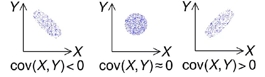
However, covariance doesn’t indicate the strength of the relationship just the direction. That's where correlation comes in (we’ll cover that next).
\text{Cov}(X, Y) = \frac{1}{n – 1} \sum_{i=1}^{n} (x_i – \bar{x})(y_i – \bar{y})
\)
import pandas as pd

# Sample data: Study hours and exam scores
study_hours = [4, 6, 8, 9, 10]
exam_scores = [60, 65, 80, 85, 90]

# Using Pandas
df = pd.DataFrame({'Study Hours': study_hours, 'Exam Scores': exam_scores})
print("Pandas Covariance:\n", df.cov())

#Output:
#               Study Hours  Exam Scores
# Study Hours         5.80        30.75
# Exam Scores        30.75       167.50
This positive covariance suggests that as study time increases, exam scores tend to increase a logical and expected relationship.
Correlation in Python: Understanding Strength and Direction of Relationships
While covariance tells you the direction of a relationship between two variables, correlation goes further by also measuring its strength. The most common correlation metric is Pearson's correlation coefficient, which is standardized and ranges between -1 and 1.
| Correlation Value | Meaning |
|---|---|
| +1 | Perfect positive correlation |
| 0 | No correlation |
| –1 | Perfect negative correlation |
So, while covariance tells you whether variables move together, correlation tells you how strongly and consistently they move together.
r = \frac{\text{Cov}(X, Y)}{\sigma_X \cdot \sigma_Y}
\)
import pandas as pd

# Data: Study hours and exam scores
study_hours = [4, 6, 8, 9, 10]
exam_scores = [60, 65, 80, 85, 90]

# Using Pandas
df = pd.DataFrame({'Study Hours': study_hours, 'Exam Scores': exam_scores})
print("Pandas Correlation:\n", df.corr())

# Pandas Correlation:
#               Study Hours  Exam Scores
# Study Hours      1.00000      0.98656
# Exam Scores      0.98656      1.00000
A correlation of 0.98 indicates a very strong positive linear relationship suggesting the more students study, the better they score.
Key Takeaways:
- Correlation is unitless, making it perfect for comparing variables on different scales.
- Pearson’s correlation assumes a linear relationship. For nonlinear or rank-based relationships, consider:
- Spearman correlation (monotonic)
- Kendall’s Tau (ordinal data)
Be Careful:
Correlation does not imply causation! Just because two variables move together doesn’t mean one causes the other.
Visualizing Correlation with a Heatmap
To better understand relationships between multiple variables, a correlation heatmap is an effective visual tool. It displays the pairwise correlation coefficients between variables in a colored matrix, making it easier to spot strong, weak, or negative correlations at a glance. Warmer colors typically represent stronger positive correlations, while cooler tones indicate negative ones.
Here’s how to generate a correlation heatmap using Seaborn in Python:
import seaborn as sns
sns.heatmap(data= df.corr(), annot=True, cmap='coolwarm', linewidths=1, linecolor='black', center=0)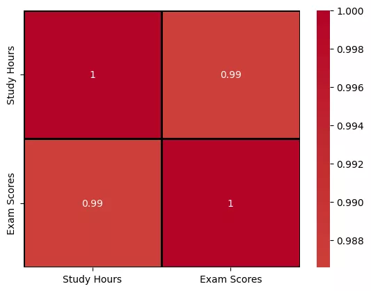
Normal Distribution in Python: The Bell Curve Explained
The normal distribution often called the bell curve is a continuous probability distribution that is symmetric around its mean. It describes how the values of a variable are distributed and is commonly found in natural and social phenomena like heights, IQ scores, and standardized test results.
Understanding this distribution is important because:
- Many statistical methods assume normality
- It helps assess skewness, outliers, and probability
- It’s the foundation of z-scores, hypothesis testing, and confidence intervals
Characteristics of a Normal Distribution
- Symmetrical around the mean
- Mean = Median = Mode
- About 68% of data falls within ±1 standard deviation
- About 95% falls within ±2, and 99.7% within ±3 (the empirical rule)
In the real world, perfect normal distributions are rare. Most datasets approximate a normal distribution but include some degree of skewness, kurtosis, or outliers.
So while your data might not follow a textbook-perfect bell curve, many statistical methods still apply as long as the deviation from normality is not too extreme.
Conclusion: Mastering Descriptive Statistics with Python
Descriptive statistics form the foundation of data analysis, allowing you to summarize, understand, and communicate the main features of your dataset before diving into complex models. In this post, we explored:
- Measures of central tendency (mean, median, mode)
- Measures of dispersion (standard deviation, variance, coefficient of variation)
- Relationships through covariance and correlation
- The role of the normal distribution in real-world data
Using Python libraries like NumPy, Pandas, Seaborn, and Matplotlib, you can efficiently compute and visualize these statistics to uncover key insights from your data.
Whether you're a data analyst, scientist, or beginner learning Python for data analysis, understanding descriptive statistics is your first step toward smarter, data-driven decisions.
This next section may contain affiliate links. If you click one of these links and make a purchase, I may earn a small commission at no extra cost to you. Thank you for supporting the blog!
References
Python for Data Analysis: Data Wrangling with pandas, NumPy, and IPython
https://www.geeksforgeeks.org/statistics-with-python
Practical Statistics for Data Scientists: 50+ Essential Concepts Using R and Python
Python 3: The Comprehensive Guide to Hands-On Python Programming
Fluent Python: Clear, Concise, and Effective Programming
Frequently Asked Questions (FAQs)
What is the difference between descriptive and inferential statistics?
Descriptive statistics summarize and describe the main features of a dataset using metrics like mean, median, and standard deviation. Inferential statistics, on the other hand, make predictions or generalizations about a population based on a sample.
When should I use median instead of mean?
Use the median when your data is skewed or contains outliers, as it better represents the center of the data in such cases. The mean can be heavily influenced by extreme values.
Can I use mode for continuous data?
Mode is best suited for categorical or discrete data. It can be calculated for continuous data, but it's often less meaningful unless the data is binned or grouped.
What does a high standard deviation indicate?
A high standard deviation means that the data points are spread out far from the mean, indicating greater variability in your dataset.
Why is the normal distribution so important?
The normal distribution appears in many natural phenomena and underpins key statistical concepts like the Central Limit Theorem, z-scores, and confidence intervals. Many statistical tests also assume normality.


