Supervised LearningLinear RegressionMachine LearningpythonRegression Analysis

Regression with scikit-learn Simplified: A practical guide for Beginners

DataLensBlogger

January 12, 2025

11 Min Read

0 Comments

Regression analysis is a cornerstone of predictive modeling in machine learning. Whether you're forecasting sales, predicting prices, or analyzing trends, regression techniques can help uncover valuable insights from your data. Among the many tools available for this purpose, Scikit-Learn stands out for its simplicity, flexibility, and power. In this blog, you'll explore how to implement regression with Scikit-Learn, covering everything from data preprocessing to model evaluation. By the end, you'll be equipped with actionable steps to build your own regression models.

What Is Regression in Machine Learning?

While classification is the problem of categorizing data into predefined classes based on input features,Regression predictive modeling involves understanding the relationship between independent variables and dependent variables by measuring the strength of their association. The target variable typically has continuous values, such as a weather conditions, stock prices, country's GDP, or housing prices.

Regression Data Set

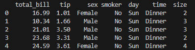
To better understand regression analysis, let’s explore a dataset that examines tips received by food servers in restaurants. This dataset includes features such as meal price, gender of the person paying the bill, whether the party included smokers, size of the dining party,time of the meal (Lunch or Dinner, categorical) and day of the week. You can access this dataset through the Seaborn library.

import seaborn as sns
import pandas as pd

# Load a Seaborn dataset (e.g., "tips") into a Pandas DataFrame
df = sns.load_dataset('tips')

# Display the first few rows of the DataFrame
print(df.head())

# Verify the type to ensure it's a Pandas DataFrame
print(type(df))  # Output: <class 'pandas.core.frame.DataFrame'>

If you'd like to test your model using other datasets available in Seaborn, you can view the complete list of datasets by running the following command:

print(sns.get_dataset_names())
# Outputs: ['anagrams', 'anscombe', 'attention', 'brain_networks', 'car_crashes', 'diamonds', 'dots', 'dowjones', 'exercise', 'flights', 'fmri', 'geyser', 'glue', 'healthexp', 'iris', 'mpg', 'penguins', 'planets', 'seaice', 'taxis', 'tips', 'titanic']

Data Preprocessing

Before building regression models, it's essential to ensure that the data is in a suitable format for modeling. In this step, you'll analyze and transform the dataset into a form that is easy to work with. We examine each column in the DataFrame for missing values (NaN) and display the count of missing entries for each column.

print(df.isna().sum())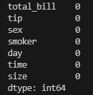

Categorical variables like sex, smoker, day, and time need to be encoded into numerical values using techniques such as one-hot encoding or label encoding.

from sklearn.preprocessing import OneHotEncoder

# One-hot encoding for categorical features
df_encoded = pd.get_dummies(df, drop_first=True)
print(df_encoded.head())

In pd.get_dummies(), the drop_first=True parameter is used to drop the first category of each categorical variable during one-hot encoding. This prevents the creation of redundant features and avoids the dummy variable trap, a situation where the encoded variables are linearly dependent.

Scikit-learn Library expects features and target values to be stored in separate variables, typically named X and y. To utilize all the features in our dataset, we begin by dropping the target column, which represents tips received by food servers in restaurants, and assign the remaining data to the variable `X` using the `values` attribute. For the target variable `y`, we extract the `values` attribute directly from the target column. We can verify that both X and y are now NumPy arrays with the same number of observations by printing their data types and shapes.

X = df_encoded.drop('tip', axis=1).values
y = df_encoded['tip'].values
print(type(X), type(y)) #Output: <class 'numpy.ndarray'> <class 'numpy.ndarray'>
print(X.shape, y.shape) #Output: (244, 8) (244,)

Performing Regression on the Tips Dataset

It is necessary to split data into a training set and a test set, to fit the Regression model using the training set,then we calculate the model performance using the test set’s labels.To split data, we import train_test_split from sklearn.model_selection.

from sklearn.model_selection import train_test_split
X_train, X_test, y_train, y_test = train_test_split(X, y, test_size=0.2, random_state=42)

We call train_test_split, passing our features and targets. Typically, 20% of the data is set aside as the test set. By specifying `test_size=0.2`, we allocate 20% of the dataset for testing. The `random_state` parameter acts as a seed for the random number generator used to split the data. Setting the same seed ensures the split and subsequent results are reproducible. To maintain accuracy, it’s considered best practice to ensure the split preserves the original proportion of labels within the dataset.

We will use linear regression to predict the tips received by restaurant food servers, leveraging all the features available in the tips dataset.

from sklearn.linear_model import  LinearRegression

linearRegression= LinearRegression()
linearRegression.fit(X_train, y_train)
y_pred= linearRegression.predict(X_test)

We imported the LinearRegression from sklearn.linear_model than we instantiate the model, fit it on the training set, and predict on the test set.

Evaluating Model Performance

The performance of a linear regression model must be meticulously evaluated to ensure its accuracy and reliability in predicting outcomes. Key metrics such as Mean Absolute Error (MAE), Mean Squared Error (MSE), and R-squared are indispensable tools in measuring how well the model fits your data. MAE provides a straightforward measure of the average error magnitude, while MSE places greater emphasis on larger errors by squaring them, offering insight into the variance of the residuals. Meanwhile, R-squared quantifies the proportion of the variance in the dependent variable that the model explains, giving a clear picture of its predictive power. By leveraging these metrics, you can identify areas needing improvement and refine the model for optimal results, ensuring it delivers precise, dependable predictions. R-squared values can range from zero to one, with one meaning the features completely explain the target's variance.

To compute R-squared, we call the model score method, passing the test features and targets. Here the features only explain about 43 percent of the tips received variance.

test_score = linearRegression.score(X_test, y_test)
print(test_score) #output: 0.43730181943482516

Another common way to evaluate the performance of a regression model is by calculating the mean of the residual sum of squares, known as the Mean Squared Error (MSE). The MSE is expressed in the squared units of the target variable. For instance, if the model predicts dollar values, the MSE will be measured in squared dollars. To interpret the error in the original units, simply take the square root of the MSE. This value is called the Root Mean Squared Error (RMSE) and provides a more intuitive measure of the model's predictive accuracy. To calculate the RMSE, we use `root_mean_squared_error` from `sklearn.metrics`. By passing `y_test` and `y_pred` as arguments , we obtain the square root of the Mean Squared Error. This gives us a clearer measure of the model's performance, revealing an average error in tips recieveid predictions of approximately 0.84 dollars.

from sklearn.metrics import root_mean_squared_error
rmse = root_mean_squared_error(y_test, y_pred )
print(rmse) #output: 0.8386635807900629

Enhancing Regression Model Performance with Cross-Validation

When calculating R-squared on a test set, the result can vary depending on how the data is split. Distinctive Features in the test data may lead to an R-squared value that doesn't accurately reflect the model's ability to generalize to new, unseen data. To address this randomness and improve reliability, we use a technique known as cross-validation. Cross-validation splits the data into multiple subsets or “folds” and trains the model on different combinations of these folds. This method helps to reduce variance in model performance estimation and prevents overfitting.

For regression tasks, common cross-validation methods include: Stratified K-Fold: Ensures proportional representation of different target ranges in each fold (less common in regression). K-Fold Cross-Validation: Divides the data into K folds and trains the model on K-1 folds while testing on the remaining fold. This process repeats K times Leave-One-Out Cross-Validation (LOOCV): Uses all data points except one for training and tests on the single remaining point.

In this guide we will perform k-fold cross-validation, There is, however, there is a trade-off to consider. Increasing the number of folds comes at a higher computational cost, as it requires performing more iterations of fitting and predicting.

from sklearn.model_selection import cross_val_score, KFold

KF= KFold(n_splits=5, shuffle=True, random_state=42)
linear_Reg = LinearRegression()
model_scores = cross_val_score(linear_Reg, X, y, cv=KF)
print(model_scores) 
#Output: [0.43730182 0.09225183 0.56146197 0.50059724 0.32369906]

To implement k-fold cross-validation using scikit-learn,we start by importing cross_val_score from sklearn.model_selection. Additionally, we import KFold to define a consistent seed and shuffle your data, ensuring reproducible results in future analyses.

We call the `cross_val_score` function by providing the model, feature data, and target data as the first three positional arguments. To define the number of folds, we pass our `KF` variable to the `cv` keyword argument. This function returns an array of cross-validation scores, which we store in the variable `model_scores`. The length of this array corresponds to the number of folds used in the process. By default, the score calculated is R-squared, as this is the standard metric for linear regression models.

Optimizing Regression Models with Regularization

Regularization is a vital technique in machine learning that enhances the performance and generalization of regression models by reducing the risk of overfitting, especially when there are many features or multicollinearity. By adding a penalty term to the regression objective function, it effectively limits the model's complexity, ensuring it remains both accurate and robust.

Ridge Regression (L2 Regularization)

Ridge regression reduces the impact of large coefficients without entirely removing features, making it an excellent choice for addressing multicollinearity by adding an L2 penalty (squared magnitude of coefficients).

When working with ridge regression, selecting the right alpha value is crucial for accurate fitting and prediction. The goal is to choose the alpha that allows the model to perform at its best. This process is comparable to selecting the optimal value of k in K-Nearest Neighbors (KNN).

When alpha is set to zero, the model performed is a simple Linear Regression model, where large coefficients are not penalized, increasing the risk of overfitting. Conversely, a high alpha imposes significant penalties on large coefficients, which can result in underfitting.

from sklearn.linear_model import Ridge

model_scores = []
for alpha in range(1, 500, 100):
    ridge= Ridge(alpha=alpha)
    ridge.fit(X_train, y_train)
    y_pred = ridge.predict(X_test)
    model_scores.append(ridge.score(X_test, y_test))

print(model_scores)
#Outputs: [0.4390233759226173, 0.5016961885929453, 0.5186831916368424, 0.52681361179751, 0.5316437950081734]

we first import the `Ridge` class from `sklearn.linear_model`. To demonstrate the effect of varying alpha values, we initialize an empty list to store our scores and define a list of alpha values to iterate through. Within the loop, we instantiate a `Ridge` model, setting the `alpha` parameter to the current value of the iterator. We then fit the model using the training data and make predictions on the test data. The model's R-squared value is calculated and appended to the scores list. After completing the loop, we print the R-squared scores for models trained with five different alpha values, providing a clear comparison of their performance.

Lasso Regression (L1 Regularization)

Lasso regression excels at both regularization and feature selection, making it an ideal choice for working with sparse datasets.

from sklearn.linear_model import Lasso

model_scores = []

for alpha in range(1, 500, 100):
    lasso= Lasso(alpha=alpha)
    lasso.fit(X_train, y_train)
    y_pred = lasso.predict(X_test)
    model_scores.append(ridge.score(X_test, y_test))

print(model_scores)
#Outputs: [0.5467115210170849, -0.15896098636013822, -0.15896098636013822, -0.15896098636013822, -0.15896098636013822]

This code demonstrates the implementation of Lasso Regression to assess model performance across various values of the regularization parameter, alpha. It calculates the model's R² scores, appends them to the `model_scores` list, and then outputs the results. From the observed outputs, it is clear that performance declines significantly after the first iteration as alpha increases.

Lasso regression is a powerful tool for assessing feature importance. By applying regularization, it shrinks the coefficients of less relevant features to zero, effectively filtering them out. Features with non-zero coefficients are identified as significant by the lasso algorithm, making it a valuable method for feature selection.

from sklearn.linear_model import Lasso
import matplotlib.pyplot as plt

lasso= Lasso(alpha=1)
features= df_encoded.drop('tip', axis=1).columns
lasso_coefficients = lasso.fit(X, y).coef_
plt.bar(features, lasso_coefficients)
plt.xticks(rotation=20)
# saving the figure. 
plt.savefig("feature_selection.png", 
            bbox_inches ="tight", 
            pad_inches = 1, 
            orientation ='landscape') 
plt.show()

We began by creating our feature and target arrays, leveraging the `pandas.DataFrame.columns` attribute to access the feature names and store them in a variable called `features`. Since we are calculating feature importance, we used the entire dataset rather than splitting it.

Next, we instantiated a Lasso regression model, setting the alpha parameter to 1. After fitting the model to the data, we extracted the coefficients using the `coef_` attribute and stored them in a variable called `lasso_coefficients`.

To visualize the results, we plotted the coefficients for each feature. Unsurprisingly, the analysis revealed that the most significant predictor of our target variable tips was the total bill. While this outcome aligns with expectations, it serves as an excellent sanity check for our approach.

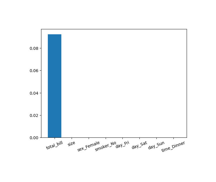
Feature selection like this is invaluable. It not only helps convey insights to non-technical audiences but also highlights the key factors driving various phenomena, making it an essential tool for both communication and discovery.

Conclusion

Regularized regression techniques like Ridge and Lasso are invaluable tools in machine learning, especially when working with datasets that have multicollinearity or numerous features. These methods not only improve the stability and performance of regression models but also help in feature selection and generalization.

Through this guide, you’ve learned:

• The concepts behind Ridge, Lasso, and Elastic Net regression.
• How to implement these techniques using Scikit-Learn.
• How to evaluate models using metrics like R² and Root Mean Squared Error (RMSE).
• How to choose the right regularization strength (alpha) and the challenges of underfitting and overfitting.

By applying these techniques and fine-tuning hyperparameters like alpha, you can build robust models that strike a balance between accuracy and simplicity.

This next section may contain affiliate links. If you click one of these links and make a purchase, I may earn a small commission at no extra cost to you. Thank you for supporting the blog!

References

Hands-On Machine Learning with Scikit-Learn, Keras, and TensorFlow

Introduction to Machine Learning with Python: A Guide for Data Scientists

Machine Learning with PyTorch and Scikit-Learn: Develop machine learning and deep learning models with Python

DATA SCIENCE THROUGH PYTHON. SUPERVISED LEARNING TECHNIQUES: kNN, SVM, NAIVE BAYES, BAGGING, BOOSTING, STACKING, AND NEURAL NETWORKS 

Python Machine Learning By Example: Unlock machine learning best practices with real-world use cases

FAQs