

Motor Vehicle Crashes remain one of the leading causes of injury and fatality in urban environments, and New York City is no exception. With thousands of crashes reported each year, understanding the patterns and factors behind these incidents is crucial for improving road safety and informing policy decisions. In this blog post, we dive deep into the NYC Motor Vehicle Crashes dataset, analyzing nearly 180,000 reported crashes to uncover when, where, and why these Vehicle Crashes occur.
Leveraging data visualization and spatial analysis techniques, we reveal key trends from temporal variations like day versus night Vehicle Crashes to hotspot mapping across boroughs. Whether you’re a data enthusiast, urban planner, or concerned citizen, this analysis provides valuable insights into NYC’s traffic safety landscape.
Table of Contents
Data Overview and Cleaning
The dataset used in this analysis, titled “Motor Vehicle Crashes”, is published by the NYC Open Data portal and contains detailed records of traffic crashes across New York City. The version used for this project includes 179,921 records and 29 columns, covering variables such as crash date and time, location (borough, ZIP code, latitude, longitude), contributing factors, vehicle types involved, and the number of persons injured or killed.
However, like most real-world datasets, this one required careful cleaning before meaningful analysis could begin.
import pandas as pd

pd.set_option('display.max_columns', None) # This allows us to view all columns in a dataframe when called
pd.set_option('display.max_rows', 300) # This returns 200 rows at max to prevent accidents when writing code
pd.options.display.max_info_rows = 1000000
data= pd.read_csv('Motor_Vehicle_Collisions_-_Crashes.csv')
print(data.info())
#Output:

# <class 'pandas.core.frame.DataFrame'>
# RangeIndex: 179921 entries, 0 to 179920
# Data columns (total 29 columns):
#  #   Column                         Non-Null Count   Dtype
# ---  ------                         --------------   -----
#  0   CRASH DATE                     179921 non-null  object
#  1   CRASH TIME                     179921 non-null  object
#  2   BOROUGH                        118160 non-null  object
#  3   ZIP CODE                       118137 non-null  float64
#  4   LATITUDE                       164788 non-null  float64
#  5   LONGITUDE                      164788 non-null  float64
#  6   LOCATION                       164788 non-null  object
#  7   ON STREET NAME                 130909 non-null  object
#  8   CROSS STREET NAME              83247 non-null   object
#  9   OFF STREET NAME                49010 non-null   object
#  10  NUMBER OF PERSONS INJURED      179920 non-null  float64
#  11  NUMBER OF PERSONS KILLED       179921 non-null  int64
#  12  NUMBER OF PEDESTRIANS INJURED  179921 non-null  int64
#  13  NUMBER OF PEDESTRIANS KILLED   179921 non-null  int64
#  14  NUMBER OF CYCLIST INJURED      179921 non-null  int64
#  15  NUMBER OF CYCLIST KILLED       179921 non-null  int64
#  16  NUMBER OF MOTORIST INJURED     179921 non-null  int64
#  17  NUMBER OF MOTORIST KILLED      179921 non-null  int64
#  18  CONTRIBUTING FACTOR VEHICLE 1  179017 non-null  object
#  19  CONTRIBUTING FACTOR VEHICLE 2  138963 non-null  object
#  20  CONTRIBUTING FACTOR VEHICLE 3  18150 non-null   object
#  21  CONTRIBUTING FACTOR VEHICLE 4  4933 non-null    object
#  22  CONTRIBUTING FACTOR VEHICLE 5  1490 non-null    object
#  23  COLLISION_ID                   179921 non-null  int64
#  24  VEHICLE TYPE CODE 1            177754 non-null  object
#  25  VEHICLE TYPE CODE 2            119747 non-null  object
#  26  VEHICLE TYPE CODE 3            16869 non-null   object
#  27  VEHICLE TYPE CODE 4            4668 non-null    object
#  28  VEHICLE TYPE CODE 5            1439 non-null    object
The output of data.info() provides a structural summary of the NYC vehicle crashes dataset. It shows that the dataset contains 179,921 rows and 29 columns, each representing different attributes of traffic collision records. This summary is essential for understanding the completeness and type of data before conducting any analysis. Here's what we can gather:
- The dataset uses a RangeIndex from 0 to 179,920 indicating no custom index is applied.
- Data types include:
object(strings or mixed types): 17 columnsfloat64: 4 columns (e.g., latitude, longitude, injuries)int64: 8 columns (e.g., fatality counts, collision ID)
- Missing values are present in several key columns:
BOROUGH,ZIP CODE,LATITUDE, andLONGITUDEhave thousands of missing entries.- Street name and contributing factor columns show even more sparsity.
- All injury and fatality-related columns are mostly complete, which is crucial for safety analysis.
This overview guides us on where to clean, convert data types, and which fields may require imputation or filtering before analysis.
Each column should contain approximately 179,920 values, though some columns have considerably fewer entries. Let's find the percentage of the missing values and see which columns have the most amount of missing values. To do so we will get a mean of the missing values and then round it to the second decimal.
print(data.isnull().mean().round(4) * 100)
#output:
# CRASH DATE                        0.00
# CRASH TIME                        0.00
# BOROUGH                          34.33
# ZIP CODE                         34.34
# LATITUDE                          8.41
# LONGITUDE                         8.41
# LOCATION                          8.41
# ON STREET NAME                   27.24
# CROSS STREET NAME                53.73
# OFF STREET NAME                  72.76
# NUMBER OF PERSONS INJURED         0.00
# NUMBER OF PERSONS KILLED          0.00
# NUMBER OF PEDESTRIANS INJURED     0.00
# NUMBER OF PEDESTRIANS KILLED      0.00
# NUMBER OF CYCLIST INJURED         0.00
# NUMBER OF CYCLIST KILLED          0.00
# NUMBER OF MOTORIST INJURED        0.00
# NUMBER OF MOTORIST KILLED         0.00
# CONTRIBUTING FACTOR VEHICLE 1     0.50
# CONTRIBUTING FACTOR VEHICLE 2    22.76
# CONTRIBUTING FACTOR VEHICLE 3    89.91
# CONTRIBUTING FACTOR VEHICLE 4    97.26
# CONTRIBUTING FACTOR VEHICLE 5    99.17
# COLLISION_ID                      0.00
# VEHICLE TYPE CODE 1               1.20
# VEHICLE TYPE CODE 2              33.44
# VEHICLE TYPE CODE 3              90.62
# VEHICLE TYPE CODE 4              97.41
# VEHICLE TYPE CODE 5              99.20
The output shows the percentage of missing (null) values in each column of the motor vehicle collision dataset. This helps assess data quality and informs decisions about which columns can be trusted, cleaned, or possibly removed. Several columns are fully complete, while others have significant gaps in coverage.
Key takeaways:
- ✅ No Missing Data (0%) in:
CRASH DATE,CRASH TIME, all injury and fatality columns (NUMBER OF PERSONS INJURED/KILLED, etc.), andCOLLISION_ID.
- ⚠️ Moderate Missing Data:
LATITUDE,LONGITUDE, andLOCATION: ~8.4% missing; crucial for mapping.BOROUGHandZIP CODE: ~34% missing; relevant for spatial and borough-level analysis.ON STREET NAME: 27.24% missing; useful for location-specific insights.
- ❗ High Missing Data:
CROSS STREET NAME: 53.73% missing.OFF STREET NAME: 72.76% missing.CONTRIBUTING FACTOR VEHICLE 3–5: over 89% missing.VEHICLE TYPE CODE 3–5: over 90% missing; often related to crashes involving more than two vehicles.
This analysis highlights which columns are reliable for analysis and which ones are too sparse to be meaningful without advanced imputation or filtering.
#Standardize Column Names
data.columns= data.columns.str.lower().str.replace(' ', '_')

#Drop Irrelevant and Highly Sparse Columns
df = data.drop(columns=['contributing_factor_vehicle_3', 'contributing_factor_vehicle_4', 'contributing_factor_vehicle_5', 'vehicle_type_code_3','vehicle_type_code_4',
'vehicle_type_code_5','on_street_name','off_street_name','cross_street_name','location'], axis=1)

#Combine Date and Time into Datetime
data['crash_datetime']= pd.to_datetime(data['crash_date'].astype(str) + ' ' + data['crash_time'] , dayfirst=True)

# Fill missing boroughs  mark as 'Unknown'
df['borough'] = df['borough'].fillna('Unknown')
We first standardize column names by converting them to lowercase and replacing spaces with underscores. This improves consistency and simplifies column referencing in later operations.
Next, we remove irrelevant or highly sparse columns such as contributing factors and vehicle types for vehicles 3–5, street names, and the redundant location field. These columns contain large amounts of missing data and are unlikely to add significant value to the analysis.
To enable more insightful time-based analysis, we combined the separate crash_date and crash_time columns into a single crash_datetime column. This transformation allows us to treat each crash as a timestamped event, making it easier to perform operations such as sorting by time, filtering by specific dates, or extracting components like the hour, day of the week, or month.
Finally, we fill missing values in the borough column with the label 'Unknown', ensuring that this important categorical variable has no null entries that could disrupt grouping or visualization tasks. This step improves both the cleanliness and usability of the dataset for further analysis and visualization.
Feature Engineering
With the dataset cleaned and standardized, the next crucial step is feature engineering by transforming raw data into meaningful variables that can reveal deeper insights.
By creating new features from existing columns, especially from the combined datetime field, we unlock the potential to analyze patterns across different times of day, days of the week, and other dimensions.
These engineered features will serve as powerful tools for both visualization and predictive modeling, helping us better understand the dynamics of motor vehicle collision in New York City.
#Temporal Features
df['hour'] = df['crash_datetime'].dt.hour
df['day_of_week'] = df['crash_datetime'].dt.day_name()
df['month'] = df['crash_datetime'].dt.month_name()
df['year'] = df['crash_datetime'].dt.year

#Injury/Killed Aggregation
df['total_injured']=df[['number_of_persons_injured', 'number_of_cyclist_injured', 'number_of_motorist_injured']].sum(axis=1)
df['total_killed']=df[['number_of_persons_killed', 'number_of_cyclist_killed', 'number_of_motorist_killed']].sum(axis=1)

#Spatial Processing
df_valid_coords = df[(df['longitude'].notnull()) & (df['latitude'].notnull())]
gdf = gpd.GeoDataFrame(df_valid_coords,
geometry=gpd.points_from_xy(df_valid_coords['longitude'], df_valid_coords['latitude'], crs='EPSG:4326'))

#Vehicle Crashes involved in by DAY/NIGHT
df['DaY/NIGHT']=  df['hour'].apply(lambda x: 'Day' if 6 <= x < 18 else 'Night')
In the code above, we engineered several new features to enhance the dataset for more insightful analysis. Starting with temporal features, we extracted the hour, day of the week, month, and year from the crash_datetime column.
These features allow us to analyze crash trends across different time intervals. We then aggregated injury and fatality data into two new columns total_injured and total_killed to simplify severity analysis.
For spatial analysis, we filtered out records with missing geographic coordinates and converted valid latitude and longitude points into a GeoDataFrame, enabling future spatial visualization and geospatial queries. Lastly, we introduced a day/night classification by categorizing each crash based on the hour it occurred, which allows us to study the impact of time-of-day on collision frequency.
Exploratory Data Analysis (EDA)
With the dataset cleaned and key features engineered, we’re now ready to dive into exploratory data analysis (EDA) the stage where we begin to uncover meaningful insights from the data. This step involves visualizing trends, examining distributions, and identifying patterns across time, location, and crash severity.
Through EDA, we aim to answer critical questions like: When do most Vehicle Crashes occur? Which boroughs are most affected? Are Vehicle Crashes more frequent during the day or night? By combining statistics and visualizations, this analysis will provide a comprehensive overview of motor vehicle collision dynamics in New York City.
#Frequency of Vehicle Crashes By Borough
print(df['borough'].value_counts())

# Number of injuries and death
print(f'Number of injuries: {df['total_injured'].sum()} \n \
      Number of deaths: {df['total_killed'].sum()}')

# Contributing Factors analysis
print(df['contributing_factor_vehicle_1'].value_counts().head(10))

# Vehicle Type Distribution related to Crashes
print(df['vehicle_type_code_1'].value_counts().head(10))

#Ouput:

# borough
# Unknown          61761
# BROOKLYN         40823
# QUEENS           31815
# BRONX            21681
# MANHATTAN        19365
# STATEN ISLAND     4476
# Name: count, dtype: int64

# Number of injuries: 155402.0
#        Number of deaths: 712

# contributing_factor_vehicle_1
# Unspecified                       44464
# Driver Inattention/Distraction    43651
# Failure to Yield Right-of-Way     12280
# Following Too Closely             11876
# Passing or Lane Usage Improper     8105
# Passing Too Closely                6946
# Unsafe Speed                       6286
# Backing Unsafely                   5704
# Traffic Control Disregarded        5068
# Other Vehicular                    4790
# Name: count, dtype: int64

# vehicle_type_code_1
# Sedan                                  85122
# Station Wagon/Sport Utility Vehicle    62844
# Taxi                                    4550
# Pick-up Truck                           3697
# Box Truck                               3078
# Bus                                     2985
# Bike                                    2575
# E-Bike                                  1541
# Motorcycle                              1481
# Tractor Truck Diesel                    1355
# Name: count, dtype: int64s
This code segment of the analysis provides a high-level overview of Vehicle Crashes in New York City, revealing critical trends and patterns. Here's a breakdown of what the code does and what the output tells us:
- Crash Frequency by Borough: The
value_counts()function was used to count Vehicle Crashes per borough. Brooklyn leads with the highest number of recorded Collisions (40,823), followed by Queens and the Bronx. Notably, 61,761 Vehicle Crashes were reported with an unknown borough, highlighting possible issues with location data reporting. - Total Injuries and Deaths: By summing up the engineered
total_injuredandtotal_killedcolumns, we learned that there were over 155,000 injuries and 712 deaths resulting from Vehicle Crashes a sobering reminder of the human cost of traffic accidents. - Top Contributing Factors: Analyzing the
contributing_factor_vehicle_1column showed that driver inattention/distraction dominate as leading cause of Vehicle Crashes accounting for more than 43651 incidents. Other common factors include failure to yield and following too closely. - Common Vehicle Types Involved: Looking into
vehicle_type_code_1, Sedans and SUVs were the most frequently involved vehicle types, far exceeding others like taxis, pickup trucks, and motorcycles. This suggests a correlation between vehicle prevalence on roads and involvement in accidents.
This initial exploration provides a strong foundation for deeper insights, such as temporal trends, spatial patterns, and severity analysis.
# plot Vehicle Crashes by hour, day of the week and month
import matplotlib.pyplot as plt

# Create a figure with 2 rows and 2 columns of subplots
fig, axes = plt.subplots(2, 2, figsize=(16, 12))
fig.suptitle('Vehicle Crash Analysis', fontsize=16)

df['hour'].value_counts().sort_index().plot(kind='bar',  ax=axes[0, 0], title='Vehicles Crashes By Hour')
axes[0, 0].set_xlabel('Hour of the Day')
axes[0, 0].set_ylabel('Number of Crashes')

df['day_of_week'].value_counts().sort_values(ascending=True).plot(kind='barh', ax=axes[0, 1], color='lightblue', edgecolor='black',title='Vehicle Crashes By Day of the Week')
axes[0, 1].set_xlabel('Number of Crashes')
axes[0, 1].set_ylabel('Day of the week')

df['month'].value_counts().sort_values(ascending=True).plot(kind='barh',ax=axes[1, 0],
title='Vehicle Crashes By Month')
axes[1, 0].set_xlabel('Number of Crashes')
axes[1, 0].set_ylabel('Month')

# Crashes count by Day/Night
day_night_crashes= df['DaY/NIGHT'].value_counts()
day_night_crashes.plot(kind='pie',  ax=axes[1, 1], autopct='%1.1f%%', colors=['orange', 'skyblue'], title='Crashes Count by Day/Night')

# Adjust layout to prevent overlapping
plt.tight_layout()
plt.subplots_adjust(top=0.92)  # Adjust for the main title
plt.show()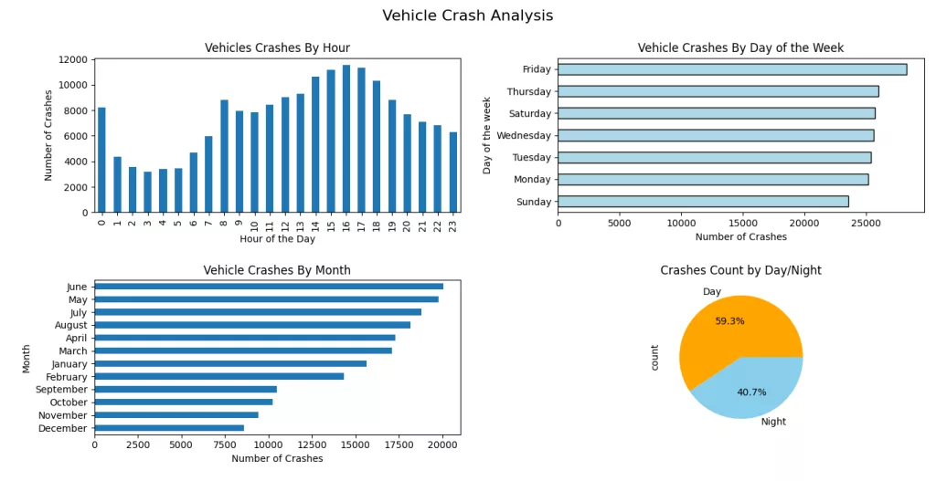
The visualization offers a clear and insightful temporal analysis of vehicle crashes in New York City, shedding light on when most accidents occur and how patterns shift across different timeframes. Here's a summary of the findings illustrated in your charts:
- Crashes by Hour: The number of vehicle crashes spikes sharply during late afternoon hours, peaking around 4–6 PM, likely due to evening rush hour traffic. A smaller peak occurs around 8 AM, indicating a morning rush hour trend.
- Crashes by Day of the Week: Fridays witness the highest number of crashes, followed closely by Thursdays and Saturdays, suggesting that the end of the workweek and weekend onset see increased traffic activity and possibly more risky driving behavior.
- Crashes by Month: The summer months, particularly June and May, record the highest crash counts. This trend might be influenced by increased travel, tourism, and more vehicles on the road during warmer months.
- Day vs Night Crashes: The pie chart reveals that 59.3% of the crashes happen during the day, while 40.7% occur at night. This indicates that despite higher visibility and possibly more traffic enforcement during daylight, a significant portion of crashes still happens during these hours likely due to volume.
Together, these visualizations highlight temporal patterns in crash occurrences and help identify critical periods for traffic safety interventions and resource allocation.
fig, axes = plt.subplots(3, 1, figsize=(16, 12))
fig.suptitle('Vehicle Crash Analysis', fontsize=16)

# Crashes per Borough
borough_crashes= df['borough'].value_counts().sort_values(ascending=True)
borough_crashes.drop('Unknown', inplace=True)
borough_crashes.plot(kind='barh',  ax=axes[0],title='Injuries and Fatalities by Borough')

#Contributing factors
contributing_factors =
df['contributing_factor_vehicle_1'].value_counts().sort_values(ascending=False).head(5)
contributing_factors.drop('Unspecified', inplace=True,errors='ignore')
contributing_factors.sort_values().plot(kind='barh', ax=axes[1], title='Top 10 Contributing Factors')

#Most Cars involved in crashes
vehicle_types= df['vehicle_type_code_1'].value_counts().head(5)
vehicle_types.sort_values().plot(kind='barh', ax=axes[2], title='Crashes Count by Vehicle Types', color= 'skyblue')

# Adjust layout to prevent overlap
plt.tight_layout()
plt.subplots_adjust(top=0.90, hspace=0.4)  # Leave space for suptitle
plt.show()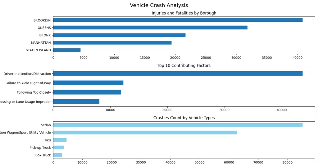
The above code snippet provides a clear and structured visualization of key factors contributing to vehicle crashes using three horizontal bar plots. Here's a breakdown of the visual analysis:
- Injuries and Fatalities by Borough:
- The first subplot shows the distribution of crashes across NYC boroughs, excluding unknown entries.
- Brooklyn has the highest number of incidents, followed by Queens, while Staten Island has the fewest.
- This may reflect traffic density and population differences across boroughs.
- Top Contributing Factors:
- The second plot highlights the top reasons for crashes.
- Driver Inattention/Distraction is by far the leading cause, significantly higher than other factors.
- Other notable causes include Failure to Yield Right-of-Way, Following Too Closely, and Improper Lane Usage.
- These insights can guide targeted traffic safety campaigns.
- Crashes Count by Vehicle Types:
- The third chart focuses on the types of vehicles most commonly involved in crashes.
- Sedans and SUVs are the top contributors, likely due to their prevalence on the roads.
- Taxis, Pick-up Trucks, and Box Trucks also appear frequently but with much lower numbers.
Overall, this multi-panel visualization provides a comprehensive snapshot of crash data, identifying where, why, and with what types of vehicles most accidents occur which is useful for urban planning, policy-making, and safety improvements.
Spatial Distribution of Vehicle Crashes
Understanding the where is just as critical as understanding the when and why in crash analysis. In this section, we explore the geographic distribution of Vehicle Crashes across the city to uncover spatial patterns and high-risk areas.
By visualizing Vehicle Crashes data on a map, we can identify hotspots, evaluate borough-level risk, and support location decision-making for traffic safety improvements. This spatial perspective not only highlights concentration zones but also informs targeted interventions for urban planners and policymakers.
gdf = gpd.GeoDataFrame(df_valid_coords, geometry=gpd.points_from_xy(df_valid_coords['longitude'], df_valid_coords['latitude'], crs='EPSG:4326'))
# Create a base map centered around NYC
map_center = [gdf['latitude'].mean(), gdf['longitude'].mean()]
crash_map = folium.Map(location=map_center, zoom_start=11, tiles='OpenStreetMap')

# Add marker clusters to avoid clutter
marker_cluster = MarkerCluster().add_to(crash_map)

# Add crash markers to the map
for _, row in gdf.iterrows():
    location = [row['latitude'], row['longitude']]
    popup_info = f"Borough: {row.get('borough', 'N/A')}<br>Injuries: {row.get('total_injured', 0)}<br>Deaths: {row.get('total_killed', 0)}"
    folium.Marker(location=location, popup=popup_info).add_to(marker_cluster)

crash_map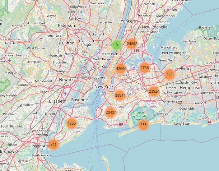
The code snippet uses GeoPandas and Folium to create an interactive map showing vehicle crash locations in New York City:
- ✅ GeoDataFrame Creation: The
gdfobject is a GeoDataFrame, built by converting latitude and longitude columns into geometrical point features. This enables spatial operations and mapping. - 📍 Map Initialization: A
folium.Mapis created and centered using the average location of all valid crash points. The map uses the OpenStreetMap tile layer for detailed basemap rendering. - 📦 Marker Clustering: To prevent overwhelming the map with thousands of individual crash markers, a
MarkerClusteris used. It groups nearby crashes into clusters, dynamically expanding as the user zooms in. - 🔍 Adding Crash Markers: Each crash point is added as a marker with a popup showing key info: borough, number of injuries, and number of deaths. This gives users interactive insight into each incident.
- 🌐 Output Map: The result is a clean, scalable visualization where crash density can be explored interactively, helping to identify crash hotspots in high-density zones like Brooklyn, Manhattan, and Queens.
Conclusion
This analysis provided a multifaceted view of vehicle crashes in New York City, combining statistical and spatial insights to understand patterns and contributing factors.
- Borough-level analysis revealed that Brooklyn and Queens experience the highest number of incidents, emphasizing the need for targeted traffic safety interventions in these areas.
- The top contributing factors such as Driver Inattention/Distraction and Failure to Yield Right-of-Way suggest that human error remains a critical challenge to road safety.
- Vehicle type analysis indicated that Sedans and SUVs are most frequently involved in crashes, possibly due to their high volume on the roads.
- Using Folium, we mapped thousands of crash locations, visualizing clusters and hotspots across the city. This spatial analysis highlights areas where crash mitigation strategies such as better signage, traffic calming, or enforcement may be urgently needed.
If you’re fascinated by the spatial dynamics of urban environments and want to dive deeper into how road network structures influence city patterns, be sure to check out our detailed blog post: Network Analysis of Paris’s Streets. It explores advanced Python techniques for uncovering hidden insights within complex street networks and offers complementary perspectives to vehicle collision studies.
In summary, this study serves as a foundation for data-driven decision-making in urban traffic management. Future work could integrate temporal patterns, weather data, or machine learning models to predict high-risk zones or times.
This next section may contain affiliate links. If you click one of these links and make a purchase, I may earn a small commission at no extra cost to you. Thank you for supporting the blog!
References
Python for Data Analysis: Data Wrangling with pandas, NumPy, and IPython
Python Data Analytics: With Pandas, NumPy, and Matplotlib
Murach's Python for Data Analysis (Training & Reference)
Frequently Asked Questions (FAQs)
What data fields were most critical in your analysis, and why?
Key fields included CRASH_DATE, CRASH_TIME for temporal analysis; LATITUDE, LONGITUDE for spatial mapping; CONTRIBUTING_FACTOR_VEHICLE_1 for causal factors; and BOROUGH to group Vehicle Crashes geographically. These fields enabled time series trends, hotspot detection, and causal pattern identification.
How was temporal analysis conducted?
Collision timestamps were parsed into datetime objects, enabling aggregation by hour, day of the week, and month. Time series decomposition and heatmaps revealed patterns like peak collision hours and seasonal variations.
How did you address missing or inconsistent data?
Records with missing coordinates or critical fields were excluded. For categorical factors, unknown or blank entries were grouped as ‘Unknown' to maintain dataset integrity. Date and time fields were validated using Python’s datetime module to catch malformed entries.
Did you incorporate external datasets or APIs in your analysis?
This analysis was limited to the NYC collision dataset, but it can be enhanced by integrating weather data (e.g., NOAA), traffic volume statistics, or road infrastructure data to model more complex causal relationships.
What dataset did you use for this analysis?
The analysis is based on the NYC Motor Vehicle Crashes dataset provided by the NYC Open Data portal. It includes detailed records of reported Vehicle Crashes in New York City, including location, date/time, contributing factors, and involved parties.


: A 101 Guide to This Simple Yet Powerful Supervised Learning Algorithm")