

Master Hypothesis Testing in Python: Step-by-Step Tutorial for Data Analysts
If you’re new to data analysis, you’ve probably heard the term hypothesis testing tossed around. But what exactly is it, and why is it so important? In simple terms, hypothesis testing is a statistical method that helps you decide whether there’s enough evidence to support a specific idea or hypothesis about your data.
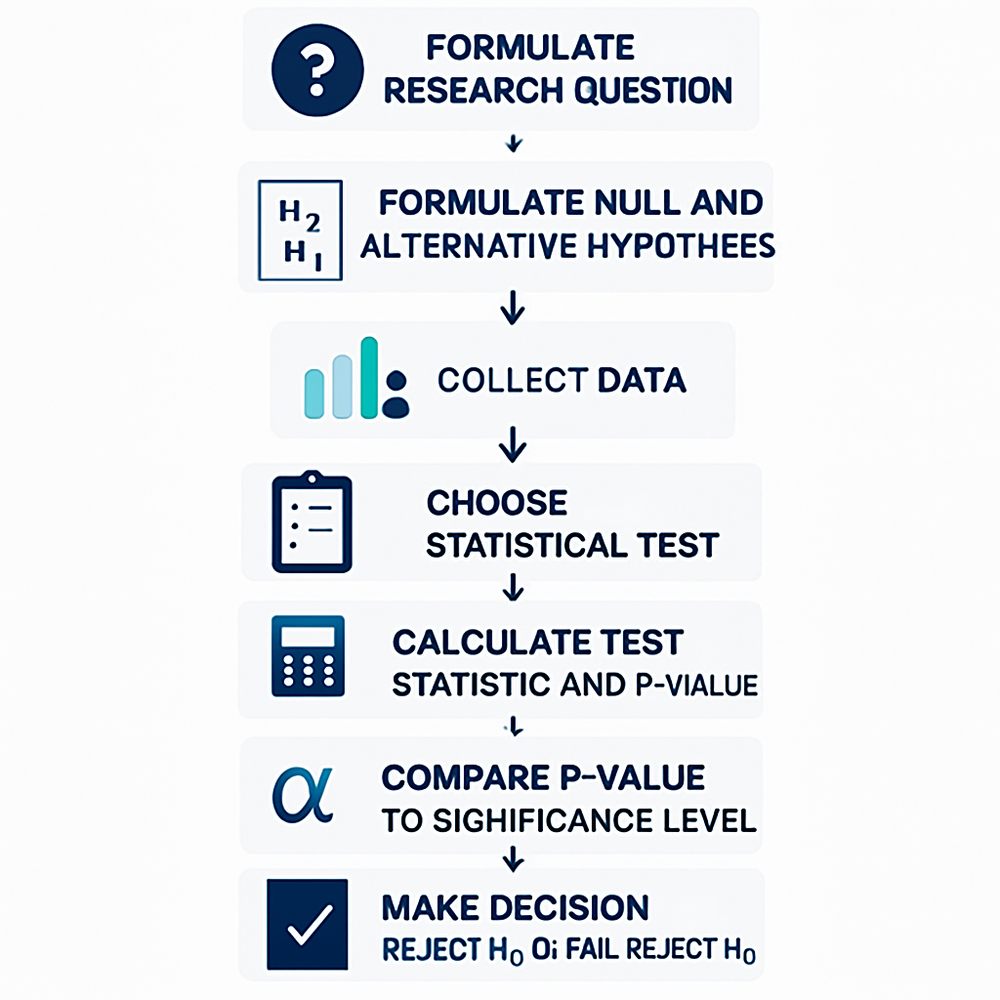
In this beginner-friendly guide, we’ll take you step-by-step through the basics of hypothesis testing from the concepts of null and alternative hypotheses to interpreting p-values. Better yet, we’ll do it all in Python, using real examples you can try right away. By the end of this post, you’ll have the practical skills and confidence to run your own hypothesis tests and make data-driven decisions like a pro.
Table of Contents
What is Hypothesis Testing?
Hypothesis testing is a fundamental technique in statistics that allows you to make decisions about data based on evidence. Imagine you have a claim for example, that a new teaching method improves students’ test scores. Hypothesis testing provides a formal process to assess whether the data you’ve collected actually supports this claim.
Here are the key ideas to understand:
- Null hypothesis (H₀): This is your baseline assumption. It usually states that there is no effect or no difference for example, that the new teaching method doesn’t change students’ scores.
- Alternative hypothesis (H₁): This is what you want to test for example, that the new teaching method does improve scores.
- Test statistic & p-value: Once you choose the appropriate test, you’ll calculate a statistic and a corresponding p-value to quantify the strength of the evidence against the null hypothesis.
- Significance level (α): A threshold (often 0.05) that tells you how strict you want to be when rejecting the null hypothesis.
By comparing your p-value to this threshold, you can decide whether to reject the null hypothesis and accept the alternative moving from raw data to a statistically justified conclusion.
What Is a p-value?
The p-value is one of the most important numbers you’ll see when you do a hypothesis test. In simple terms, it tells you:
How surprising your data would be if the null hypothesis were actually true.
More specifically:
- A small p-value (typically less than your chosen significance level, often α = 0.05) means that the observed result is unlikely under the null hypothesis.
This gives you evidence to reject the null hypothesis in favor of the alternative. - A large p-value means your data is not surprising under the null hypothesis.
This means you do not have enough evidence to reject the null hypothesis your observed difference could easily happen by random chance.
Think of the p-value as a probability score: the lower it is, the more reason you have to believe that your observed effect is real rather than a fluke.
Imagine you test whether a coin is fair by flipping it 100 times and seeing 70 heads. If the p-value is very small (e.g. 0.002), it suggests that 70 heads is very unlikely for a fair coin and you’d conclude the coin is probably biased. If the p-value is large (e.g. 0.4), then 70 heads could easily happen by chance and there’s not enough evidence to say the coin isn’t fair.
Type I and Type II Errors
When performing a hypothesis test, there are two kinds of mistakes you might make:
| Error Type | What Happens? | Example |
|---|---|---|
| Type I Error (False Positive) | Rejecting the null hypothesis when it’s actually true. | Concluding a coin is biased when it’s actually fair. |
| Type II Error (False Negative) | Failing to reject the null hypothesis when the alternative is true. | Concluding a coin is fair when it’s actually biased. |
The significance level (α) you choose often 0.05 directly controls your risk of making a Type I error. A smaller α means you’ll make fewer false positives, but that also increases the chance of a Type II error.
And here’s the key trade-off:
- Reducing Type I errors (by setting a very small α) → Increases the risk of missing a real effect (Type II errors).
- Reducing Type II errors (by increasing sample size or power) → Makes your tests more sensitive to real effects.
One-Tailed vs. Two-Tailed Tests
Two-Tailed Test
A two-tailed test checks for differences in both directions greater or smaller than the hypothesized value. Your hypotheses look like:
You’d use this when you simply want to detect any significant difference, regardless of direction.
One-Tailed Test
A one-tailed test checks for a difference in a specified direction only either greater than or less than the hypothesized value.
Two types of one-tailed tests:
Right-tailed:
Left-tailed:
Why Choose One vs. Two-Tailed?
- Use a two-tailed test if you have no prior expectation about the direction of the difference.
- Use a one-tailed test if you have a specific directional hypothesis and only care about one extreme.
Hypothesis Testing with known variance
When you know the population variance (σ²) or, equivalently, the standard deviation (σ) you can use a z-test. The z-test is a straightforward way to check whether your sample mean differs significantly from the hypothesized mean.
When to Use a z-Test
Use a z-test when:
- You know the population standard deviation (σ).
- Your sample size is large enough (usually n ≥ 30) so the Central Limit Theorem applies.
- The underlying data are approximately normally distributed.
Test Statistic Formula
The z-score is calculated as:
z = \frac{\bar{x} – \mu_0}{\sigma / \sqrt{n}}
\)
Where:
\(\begin{aligned}
\bar{x} \;&=\; \text{sample mean} \\
\mu_0 \;&=\; \text{hypothesized population mean} \\
\sigma \;&=\; \text{known population standard deviation} \\
n \;&=\; \text{sample size}
\end{aligned}
\)
Decision Rule
You compare the computed z-value to a critical z-value (based on α) or use its p-value:
- If p-value < α, reject the null hypothesis.
- Otherwise,we do not reject the null hypothesis.
Python Example
Here’s a quick example in Python. Suppose we want to test if the average weight of apples is 150 grams, knowing the standard deviation is 10 grams, and we have a sample of 50 apples with a mean weight of 153 grams.
from math import sqrt
import scipy.stats as stats

# Given data
sample_mean = 153
pop_mean = 150
pop_std = 10
n = 50
tails=2
confidence_Level= 0.95
alpha= 1-confidence_Level
# Compute z-score
z_score = (sample_mean - pop_mean) / (pop_std / sqrt(n))

# Two-tailed p-value
p_value = (stats.norm.sf(abs(z_score)))*tails

print(f"z-score: {z_score:.2f}")
print(f"p-value: {p_value:.4f}")

# Decision at alpha
if p_value < alpha:
    print("Reject the null hypothesis,  there is evidence the true mean differs from 150 g.")
else:
    print("Do not reject the null hypothesis, not enough evidence that the mean differs from 150 g.")

#output:
# z-score: 2.12
# p-value: 0.0339
# Reject the null hypothesis, there is evidence the true mean differs from 150 g.If the p-value is very small, it suggests our sample mean is unlikely if the true mean were really 150 grams so we conclude that the apples probably don’t weigh 150 grams on average. Otherwise, we don’t have enough evidence to say they differ.
Hypothesis Testing with Unknown Population Variance
In many real-world cases, we don’t know the true population standard deviation (σ). When this happens especially for smaller sample sizes we use a t-test instead of a z-test. The t-test accounts for the extra uncertainty by using the sample standard deviation (s), and it follows a t-distribution rather than the standard normal.
Test Statistic Formula
When the population standard deviation is unknown, the t-statistic is calculated as:
t = \frac{\bar{x} – \mu_0}{s/\sqrt{n}}
\)
Where:
\(\begin{aligned}
\bar{x} \;&=\; \text{sample mean} \\
\mu_0 \;&=\; \text{hypothesized population mean} \\
s \;&=\; \text{sample standard deviation} \\
n \;&=\; \text{sample size}
\end{aligned}
\)
Degrees of Freedom
With a t-test, the shape of the t-distribution depends on the degrees of freedom:
df = n – 1
$$
As your sample size grows, the t-distribution approaches the normal distribution which is why z-tests and t-tests give similar results with large samples.
Example: Testing Average Battery Life
Imagine you manufacture a phone and you claim the average battery life is 10 hours. To check this, you test a sample of 8 phones and record their battery lives (in hours):
You want to know is there enough evidence that the true mean is different from 10 hours? Let’s do a t-test by hand.
import pandas as pd
import scipy.stats as stats
import math

# Our data
data = pd.Series([9.5, 10.2, 9.7, 8.9, 10.1, 9.8, 9.4, 10.0])
pop_mean = 10.0
n = len(data)
df = n - 1
tails = 2

# Compute mean and std
sample_mean = data.mean()
s = data.std(ddof=1)

# Compute t statistic
t_stat = (sample_mean - pop_mean) / (s / math.sqrt(n))

# Compute two-tailed p-value
p_value = stats.t.sf(abs(t_stat), df) * tails

print(f"Sample mean: {sample_mean:.3f}")
print(f"Sample std dev: {s:.3f}")
print(f"t-statistic: {t_stat:.3f}")
print(f"p-value: {p_value:.3f}")

if p_value < 0.05:
    print("Reject the null hypothesis, the mean is significantly different from 10.0")
else:
    print("Fail to reject the null hypothesis, insufficient evidence of a difference")

#Output:
# Sample mean: 9.700
# Sample std dev: 0.428
# t-statistic: -1.984
# p-value: 0.088
# Fail to reject the null hypothesis, insufficient evidence of a differenceUsing scipy.stats.ttest_1samp() for a t-Test
If you’d prefer a faster and more straightforward approach, scipy.stats.ttest_1samp() can do all the heavy lifting for you in a single function call. This is ideal for real-world analyses where you want to focus on interpreting results rather than manual calculations.
Here’s the same test as before checking if the average battery life is different from 10.0 hours using ttest_1samp():
from scipy import stats
import pandas as pd

# Our data
data = pd.Series([9.5, 10.2, 9.7, 8.9, 10.1, 9.8, 9.4, 10.0])
pop_mean = 10.0

# Do it with the function
t_test, p_value = stats.ttest_1samp(data, pop_mean, alternative='two-sided')

print(f"t-statistic: {t_test:.3f}")
print(f"p-value: {p_value:.3f}")

if p_value < 0.05:
    print("Reject the null hypothesis, the mean is significantly different from 10.0")
else:
    print("Fail to reject the null hypothesis, insufficient evidence of a difference")

#Ouput:
#Fail to reject the null hypothesis, insufficient evidence of a differencePaired t-Test (Dependent Samples)
In many real-world scenarios, we want to compare measurements taken from the same subjects under two different conditions, for example:
- Measuring a person’s weight before and after starting a diet,
- Testing a machine’s accuracy before and after calibration,
- Measuring student scores before and after a training program.
In these cases, we use a paired t-test.
Why Paired?
A paired t-test accounts for the fact that the two measurements come from the same subject. Instead of looking at two separate independent groups, we look at the difference for each subject and test whether the average difference is zero.
Paired t-Test Formula
First, compute the difference for each pair:
d_i = x_{i,\text{after}} – x_{i,\text{before}}
\)
Where:
\(\begin{aligned}
x_{i, \text{after}} & = \text{the measurement for the } i\text{-th subject after the treatment} \\
x_{i, \text{before}} & = \text{the measurement for the } i\text{-th subject before the treatment}
\end{aligned}
\)
Then, apply a one-sample t-test on these differences:
Where:
\(\begin{aligned}
\bar{d} &= \text{mean of the differences } (d_i) \\
s_d &= \text{standard deviation of the differences } (d_i) \\
n &= \text{number of pairs}
\end{aligned}
\)
Python Example
Here’s a quick Python example using scipy.stats.ttest_rel():
from scipy import stats
import pandas as pd

# Paired measurements
before = pd.Series([50, 52, 48, 47, 49])
after = pd.Series([53, 54, 49, 50, 51])

# Paired t-test
t_stat, p_value = stats.ttest_rel(before, after, alternative='two-sided')

print(f"t-statistic: {t_stat:.3f}")
print(f"p-value: {p_value:.3f}")

if p_value < 0.05:
    print("Reject the null hypothesis, the mean difference is significant")
else:
    print("Fail to reject the null hypothesis, not enough evidence of a significant difference")

#Output:
# t-statistic: -5.880
# p-value: 0.004
# Reject the null hypothesis, the mean difference is significantTwo Sample T-Test (Independent Samples) with Variance Check
When you want to compare the means of two independent groups to see if they differ significantly, you use a two sample t-test (also called an independent t-test). This test helps answer questions like:
- Do men and women differ in average height?
- Is the average test score different between two classes?
- Does drug A perform differently from drug B on average?
Key assumptions for the two-sample t-test typically include:
•Independence of Observations: The data points in one group must be independent of the data points in the other group.
•Normality: The data in each group should be approximately normally distributed. While the t-test is robust to minor deviations from normality, especially with larger sample sizes, severe non-normality can affect the validity of the results.
•Homogeneity of Variances (for the standard Student's T-Test): The variances of the two populations from which the samples are drawn are assumed to be equal. This is a crucial assumption that often dictates which version of the two-sample t-test you should use.
Understanding these assumptions, particularly the last one, is critical for correctly applying the two-sample t-test and interpreting its results.
The Importance of Variance: Homoscedasticity vs. Heteroscedasticity
When comparing two group means, one of the most critical considerations is whether the variability (variance) within each group is similar or different. This concept is known as homoscedasticity (equal variances) versus heteroscedasticity (unequal variances).
•Homoscedasticity: This assumption implies that the spread of data points around the mean is roughly the same for both groups. If this assumption holds true, the standard Two Sample T-Test (often referred to as Student's T-Test) is appropriate. This version of the t-test pools the variances of the two groups to estimate the common population variance, leading to a more powerful test when the assumption is met.
•Heteroscedasticity: This occurs when the variances of the two groups are significantly different. Ignoring unequal variances and proceeding with Student's T-Test can lead to inaccurate results, specifically an inflated Type I error rate (rejecting a true null hypothesis more often than the chosen alpha level). In such cases, Welch's T-Test is the appropriate alternative. Welch's T-Test is a modification of the t-test that does not assume equal variances. It adjusts the degrees of freedom to account for the unequal variances, making it more robust and reliable when homoscedasticity is violated.
The decision of whether to use Student's T-Test or Welch's T-Test hinges entirely on the assessment of variance equality. Therefore, before performing a two-sample t-test, it is crucial to formally test for the equality of variances. This brings us to Levene's Test, a widely used method for this purpose.
Levene's Test: Checking for Equality of Variances
Before deciding between Student's T-Test and Welch's T-Test, you need a reliable way to check if the variances of your two groups are equal. This is where Levene's Test comes in. Levene's Test is a statistical test used to assess the equality of variances for a variable calculated for two or more groups. It is less sensitive to departures from normality than other tests like Bartlett's test, making it a more robust choice for many real-world datasets.
The null and alternative hypotheses for Levene's Test are:
•Null Hypothesis (H₀): The variances of the populations from which the samples are drawn are equal.
•Alternative Hypothesis (H₁): The variances of the populations from which the samples are drawn are not equal.
Levene's Test works by performing an ANOVA (Analysis of Variance) on the absolute differences between each data point and its group median (or mean, though median is generally preferred for robustness).
A small p-value (typically less than your chosen significance level, e.g., 0.05) from Levene's Test indicates that you should reject the null hypothesis, meaning there is significant evidence that the variances are unequal (heteroscedasticity). Conversely, a large p-value suggests that you fail to reject the null hypothesis, implying that the variances can be considered equal (homoscedasticity).
Python Implementation: Two Sample T-Test with Levene's Test
In Python, the scipy.stats module provides the levene function, which makes it straightforward to perform this test.
from scipy import stats
import pandas as pd

# Sample data for two independent groups
group1 = pd.Series([85, 90, 88, 75, 95])
group2 = pd.Series([80, 78, 85, 82, 79])

# Step 1: Levene's test for equal variances
levene_stat, levene_p = stats.levene(group1, group2)
print(f"Levene’s test p-value: {levene_p:.3f}")

if levene_p < 0.05:
    print("Reject the null hypothesis, Variances are unequal, perform Welch's T-Test")
else:
    print("Fail to reject the null hypothesis, Variances are equal, perform 2-sample T-Test")

# Step 2: Choose t-test type based on Levene's result
if levene_p > 0.05:
    # Variances are equal, use standard independent t-test
    t_stat, p_value = stats.ttest_ind(group1, group2, equal_var=True)
    print("Using standard independent t-test (equal variances assumed)")
else:
    # Variances are unequal, use Welch's t-test
    t_stat, p_value = stats.ttest_ind(group1, group2, equal_var=False)
    print("Using Welch’s t-test (unequal variances)")

print(f"t-statistic: {t_stat:.3f}")
print(f"p-value: {p_value:.3f}")

if p_value < 0.05:
    print("Reject the null hypothesis, the group means are significantly different")
else:
    print("Fail to reject the null hypothesis, insufficient evidence of a difference")

#Output:
# Levene’s test p-value: 0.256
# Fail to reject the null hypothesis, Variances are equal, perform 2-sample T-Test
# Using standard independent t-test (equal variances assumed)
# t-statistic: 1.634
# p-value: 0.141
#Fail to reject the null hypothesis, insufficient evidence of a differenceChi-Square Test (For Categorical Data)
So far, we've looked at hypothesis tests for numerical data (like means with t-tests). But what if your data is categorical for example, product preference, gender, region, or brand choices?
This is where the Chi-Square Test comes in. It helps you test whether:
- A categorical variable follows a certain distribution (Goodness-of-Fit), or
- Two categorical variables are associated or independent (Test of Independence).
Python implementation of Chi-Square Test
This test helps determine whether two categorical variables are statistically independent. You typically use a contingency table (cross-tab) for this.
Let’s say we want to know if product preference depends on region:
import pandas as pd
import  scipy.stats as stats

# Contingency table: Region (rows) vs. Product preference (columns)
data = pd.DataFrame({
    'Product A': [30, 20, 25],
    'Product B': [20, 25, 30],
    'Product C': [25, 30, 20]
}, index=['North', 'South', 'East'])

# Perform Chi-Square Test of Independence
chi2, p, dof, expected = stats.chi2_contingency(data)

print(f"Chi-square statistic: {chi2:.3f}")
print(f"Degrees of freedom: {dof}")
print(f"p-value: {p:.3f}")

if p < 0.05:
    print("Reject the null hypothesis, product preference depends on region.")
else:
    print("Fail to reject the null, no significant relationship between region and preference.")

#Output:
# Chi-square statistic: 6.000
# Degrees of freedom: 4
# p-value: 0.199
# Fail to reject the null, no significant relationship between region and preference.Summary
Use a Chi-Square Test when your data is categorical:
| Test Type | Use Case | Function |
|---|---|---|
| Goodness-of-Fit | Is one variable distributed as expected? | scipy.stats.chisquare |
| Test of Independence | Are two categorical variables related? | scipy.stats.chi2_contingency |
Conclusion
Hypothesis testing is a foundational tool in data analysis, allowing you to make informed decisions based on data rather than guesswork. In this post, we explored the essential types of hypothesis tests you’ll encounter when analyzing data with Python:
- One-Sample t-Test: Testing a sample mean against a known population mean.
- Paired t-Test: Comparing means from two related groups or repeated measures.
- Two-Sample t-Test: Assessing whether two independent groups have different means, with attention to variance equality.
- Chi-Square Test: Evaluating relationships and distributions in categorical data.
By understanding when and how to apply each test, as well as how to interpret p-values and test statistics, you can confidently validate hypotheses and draw meaningful conclusions from your data.
Python’s libraries like pandas and scipy.stats make implementing these tests straightforward, whether you want to compute test statistics manually or leverage built-in functions for efficiency.
Remember to always consider the nature of your data and the question at hand when choosing the right test. Also, deciding between one-tailed and two-tailed tests can significantly impact your results, so choose carefully based on your hypothesis.
With these tools and concepts in your analytical toolkit, you’re well-equipped to perform rigorous and insightful statistical analysis in Python.
This next section may contain affiliate links. If you click one of these links and make a purchase, I may earn a small commission at no extra cost to you. Thank you for supporting the blog!
References
Python for Data Analysis: Data Wrangling with pandas, NumPy, and IPython
Python Data Analytics: With Pandas, NumPy, and Matplotlib
Murach's Python for Data Analysis (Training & Reference)
Practical Statistics for Data Scientists: 50+ Essential Concepts Using R and Python
Frequently Asked Questions (FAQs)
What is the difference between a one-tailed and two-tailed test?
A one-tailed test checks for an effect in a specific direction (greater than or less than), while a two-tailed test checks for any difference regardless of direction.
When should I use a paired t-test instead of a two-sample t-test?
Use a paired t-test when the two samples are related or matched (e.g., measurements before and after on the same subjects). Use a two-sample t-test for comparing two independent groups.
What does the p-value tell me?
The p-value indicates the probability of observing your data (or something more extreme) assuming the null hypothesis is true. A small p-value (typically < 0.05) suggests evidence against the null hypothesis.
How do I decide between using the standard two-sample t-test and Welch’s t-test?
First, perform Levene’s test to check if variances are equal. If variances are equal, use the standard t-test (equal_var=True). If not, use Welch’s t-test (equal_var=False).
What assumptions do these tests make?
Common assumptions include independence of observations, normally distributed populations (especially important for small samples), and for t-tests, homogeneity of variances (for the standard two-sample test).


No Comment! Be the first one.